Text Classification using GZIP+KNN Overview
With the rise of AI in the last year, many people felt like it’s the end of creativity. There are thoughts that in the not-so-distant future AI will replace us and we’ll be out of jobs and out of purpose. AI swept over the art scene (DALL-E 2, Stable Diffusion), had some major advancement in the music scene (AI Assisted Drake Song), and even some disruptive advancements in the algorithmic scene (AI learns to multiply matrices).
I’m relatively optimistic about the impact of AI on our life, and I’m not convinced that AI will easily replace us in the foreseeable future. To strengthen this position, I’d like to walk you through recent work on text classification using GZIP compression. This paper shows us that in spite of the current trend of bigger neural networks we shouldn’t give up on trying alternative methods.
In this post I will go over the paper and the knowledge needed to understand it. In the end, I present a few of my own findings that I find quite interesting. So, even if you already know what the paper is about, make sure to read through to the end 😊.
All the code I use is available on my GitHub
Overview
In the paper “Low-Resource” Text Classification: A Parameter-Free Classification Method with Compressors the authors present a novel method to classify text using GZIP.
Their method ticks all the right boxes to make it worth checking out.
- Can be described in 14 lines of python? ✅
- On par performance with BERT? ✅
- Requires less compute and memory than current SOTA methods? ✅
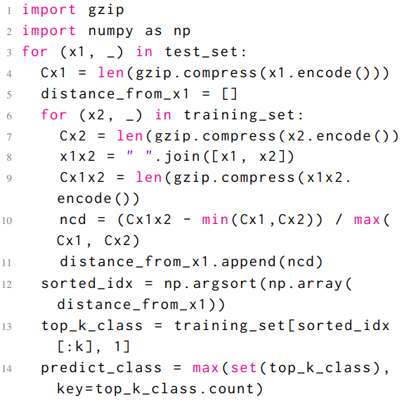
Python Code for Text Classification with GZIP. taken from the article.
Just to be clear, text classification is about classifying texts into topics (e.g., finance, engineering or music), as opposed to, let’s say, emotional classification, where the purpose is to classify the text into an emotion (e.g., positive or negative).
As for how good it is, I’ll let you see for yourselves:
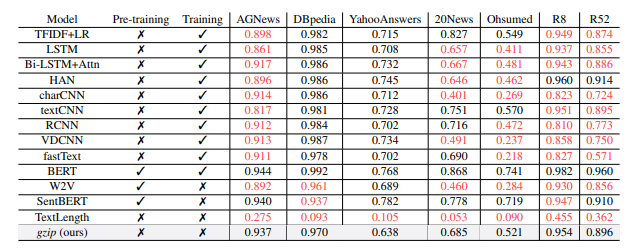
The performance of every method they tested on different datasets. Red means GZIP is better than the proposed method.
Well, looks cool on paper, but let’s dive deeper 🤿.
Basic Intuition Behind Compression
It all starts with compression. The most basic thing to understand about compression is that the more repetitions a string has, the better we can compress it. In fact, compression algorithms are sometimes used to test how much information a text contains. The intuition is if it compresses well, it doesn’t have that much information. Take a look at this very nice visualization of compression on famous pop songs. We didn’t need a compression algorithm to know some of these are very redundant, but it’s nice to be able to put a number on it.
Now that we understand that text with many repetitions compresses well, we can use this attribute of compression algorithms to test whether a string x2 adds any information to a string x1.
Let x1 and x2 be two strings. We define Cx1 and Cx2 as the compressed length of x1 and x2.
import gzip
Cx1 = len(gzip.compress(x1.encode()))
Cx2 = len(gzip.compress(x2.encode()))
And we also calculate Cx1x2 which is the compressed length of concatenated x1 and x2.
Cx1x2 = len(gzip.compress(x1+x2).encode())
If x2 does not add any new information to x1, the size of Cx1x2 should be close to the size of Cx1 or Cx2, as it will have many repetitions, and it will compress well.
On the other hand, if x1 and x2 differ significantly in content, the size of Cx1x2 would be greater, as there will not be many repetitions.
This is probably the most important point to understand to move forward, so I’ll try to explain it in simpler terms:
-
If there are many repetitions in
x1+x2, then it will compress well, andCx1x2will be small. -
If there are few repetitions in
x1+x2, it will compress poorly, andCx1x2will be large.
Example
Let’s take the following two strings:
x1 = "I ate an apple"
x2 = "I ate an apple cake"
We can see that the sentences are very similar, let’s calculate their compressed length.
Cx1 = len(gzip.compress(x1.encode())) # result is 34
Cx2 = len(gzip.compress(x2.encode())) # result is 39
Cx1x2 = len(gzip.compress((x1+x2).encode())) # result is 42
And now let’s take a third string x3
x1 = "I ate an apple"
x3 = "I walk to the park"
Cx1 = len(gzip.compress(x1.encode())) # result is 34
Cx3 = len(gzip.compress(x3.encode())) # result is 38
Cx1x3 = len(gzip.compress((x1+x3).encode())) # result is 52
We can see that even though the compressed length of x3 was smaller than x2, because x3 introduced new information to x1, we get that Cx1x3 (52) is greater than Cx1x2 (42).
In my opinion, this is the core essence of the paper, so I hope my explanation got through to you.
Pretty cool, isn’t it? 😎
Distance Function
Now that we have a basic understanding, we can define a distance function as such:
def normalized_compressed_distance(x1, x2):
	Cx1 = len(gzip.compress(x1.encode()))
	Cx2 = len(gzip.compress(x2.encode()))
	Cx1x2 = len(gzip.compress(x1+x2).encode())

	return (Cx1x2 - min(Cx1, Cx2)) / max(Cx1,Cx2)
The last line of the function is used to normalize the compression distance, so it will return a value between 0 and 1.
A value close to 1 means that the input string x1 and x2 are different (large distance).
A value close to 0 means that the input strings x1 and x2 are similar (small distance).
The Math Behind It
As explained in the paper:
Kolmogorov complexity, $K(x)$, is the length of the shortest computer program that can generate $x$. $K(x)$ is theoretically the ultimate lower bound for information measurement, as it defines the data by the smallest program that can generate it, and not by the data itself.
Take for example the following function:
def generate_data():
    return "a" * (2**30)
The data generated by this function will weigh 1GiB, but to represent that entire 1GiB of memory we only need ~40 bytes (depends if you use tabs or spaces 🕵️♀️). You might think to yourself, “but wait, the length of the program depends on the language we choose!”
Well that’s true, but the language we choose affects the length of the program up to a constant. That constant depends on the syntax of the chosen language. This is called the Invariance Theorem, and for the sake of actually finishing writing this post, I will not expand on it.
So now that we understand Kolmogorov Complexity, we can derive a distance function from it. Given two sequences $x$, $y$ where $K(y) ≥ K(x)$ we can define Normalized Information Distance as such:
\[NID(x,y) = \frac{K(y|x)}{K(y)}\]Where $K(y|x)$ is the smallest program that can generate $y$ given $x$, or in other words, the information distance between $K(y)$ and $K(x)$. Therefore if $x = y$ then $K(y|x)= 0$ the distance would be 0 and if $x$ and $y$ are independent variables then $K(y|x) = K(y)$ and the distance would be 1.
This is where we go back to the real world.
Since Kolmogorov Complexity is a theoretical limit and we have no means to calculate it exactly, the paper authors use the Normalized Compression Distance defined above as a means to approximate it.
Putting It All Together With KNN
Now that we have a way to calculate the distance between two text samples, the next thing to do is to generate a prediction. For that we will use KNN (K-nearest neighbors). Simply put, KNN uses the idea that if most of a sample’s K neighbors have a certain label, then that sample is likely to share that label.
The training set in KNN is the ground truth we use to label new samples.
For any new prediction, we measure the distance from all samples in the training set and take the K nearest neighbors.
One common way to generate a prediction is to use a simple majority vote.
In the following picture for k=3 the prediction will be ‘red triangle’, and for k=5 and the prediction will be ‘blue square’.
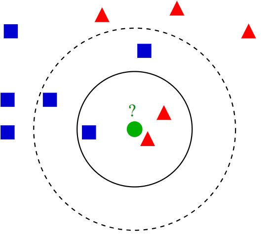
Taken from the KNN Wikipedia page.
And what do we do if there’s a tie? Well… that depends on the implementation. For example the official documentation of KNeighborsClassifier in sklearn has the following warning:
Regarding the Nearest Neighbors algorithms, if it is found that two neighbors,
neighbor `k+1` and `k`, have identical distances but different labels,
the results will depend on the ordering of the training data.
Don’t worry, we will soon deal this edge-case.
But Does it Work?
For testing purposes, all the code I used is available on GitHub.
I was honestly really excited to test it, so I decided to compare it with the model that had the best result in the paper, which was BERT.
BERT is a Large Language Model (LLM) which was introduced in 2018 by researchers at Google. At the time of it’s release it was the best model for NLP related tasks,
and even though the field of NLP saw a lot of progress since then, BERT is still sufficient for many NLP related tasks.
I also used the dataset AGNews for comparison. It wasn’t a smart and well-thought-out decision, it was just the first dataset on the performance comparison table. I could have chosen any other dataset.
I finetuned BERT on the dataset for 1 epoch with a batch size of 128 and learning rate of 2e-5.
The authors of the paper used 5 epochs with the same parameters, but I got pretty similar results.
I also used fp16 and torch.backends.cuda.matmul.allow_tf32 = True to speed up the training process.
And after 1 hour of finetuning BERT I got an accuracy score of 0.939, while the authors of the paper got 0.944.
Close enough!
Then I went on to implement my own version of GZIP+KNN, the authors use k=2 for the accuracy score, and after playing with it for a while I got the result of 0.876.
Not bad!!
But still this is a significant difference than the reported 0.937.
So what’s going on?
Well, as opposed to the regular way of predicting (e.g., majority vote) with some kind of heuristic for tie-breaking, when calculating accuracy the authors took both labels into consideration in the following way:
Let’s mark the correct label as T (for True) and the wrong label as F (for False).
| First Label | Second Label | Output |
|---|---|---|
| F | F | F |
| T | F | T |
| F | T | T |
| T | T | T |
This means that when calculating the accuracy, if the correct label is in the top 2 neighbors, we mark this as correct.
For comparison this is how I predicted the label in my implementation:
| First Label | Second Label | Output |
|---|---|---|
| F | F | F |
| T | F | T |
| F | T | F |
| T | T | T |
This means that, if there’s a tie, take the first label (as it’s the closest).
I decided not to implement the accuracy score as the authors did, because in my opinion, their way of calculating accuracy doesn’t fit with how this would be used in the real world.
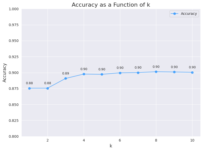
The highest accuracy received was for k=8 which was 0.9013 but as you can see the differences are pretty minor for k>=4 .
As for prediction time, using all the training set is quite compute heavy, and on my I9-12900K it takes around 15 minutes to evaluate the test set.
On the other hand, using BERT with my GeForce RTX 3060 GPU takes about a minute to evaluate the test set.
This might not seem like a straightforward comparison since I did fine-tune BERT for about an hour, and I didn’t need to do any training with the GZIP+KNN method, but for real world applications, prediction times matter a lot.
Using the GZIP+KNN method with your entire training set is quite costly, and the main reason for that is that we need to evaluate the NCD between the test sample and the entire training set.
So in conclusion, does it work? Yes, but not as advertised.
A Few Caveats
Semantic difference
While this method is pretty good for text classification, as different topics use different vocabulary, I would not use it to classify emotion as a small addition could change the entire sentence’s meaning.
Take for example the following two strings:
x1 = "I liked the movie"
x2 = "I disliked the movie"
These two strings are very similar but have a very different meaning. The method presented by the authors doesn’t give different words different impacts and treats every character the same. In this example the words ‘I’, ‘the’, ‘movie’ don’t matter for the emotion classification and only the word ‘liked’ or ‘disliked’. For these reasons I believe this method will also have difficult problems understanding sarcasm.
Possible Unintentional Bias Term?
One thing that struck me as weird is the usage of the GZIP compressed buffer as-is. The compressed buffer contains 20 bytes of metadata that are important for the algorithm for decompression, but that metadata is not part of the textual information.
When calculating the normalized compressed distance, we’re effectively bringing all samples closer together by leaving the metadata in the calculation.
Check the following code with comments:
def normalized_compressed_distance(x1, x2):
	Cx1 = len(gzip.compress(x1.encode()))
	Cx2 = len(gzip.compress(x2.encode()))
	Cx1x2 = len(gzip.compress(x1 + x2).encode())

	# 20 bytes of metadata are canceled with each other
	numerator = Cx1x2 - min(Cx1, Cx2)

	# +20 bytes of metadata
	denominator = max(Cx1,Cx2)

	# division with denominator that is bigger than should be
	return numerator / denominator
To be clear if Cx1 is greater than Cx2 then we get:
\(NCD(x_1,x_2) = \frac{Cx_1x_2-Cx_1}{Cx_2+20}\)
This also impacts the distances in a non-linear way, which means that short samples are hurt the most by the bias.
I went on to test the GZIP+KNN method with various bias terms.
I didn’t change the original implementation (GitHub), I just added a different constant in the denominator in every calculation so -20 actually means without the metadata and 0 is the original implementation
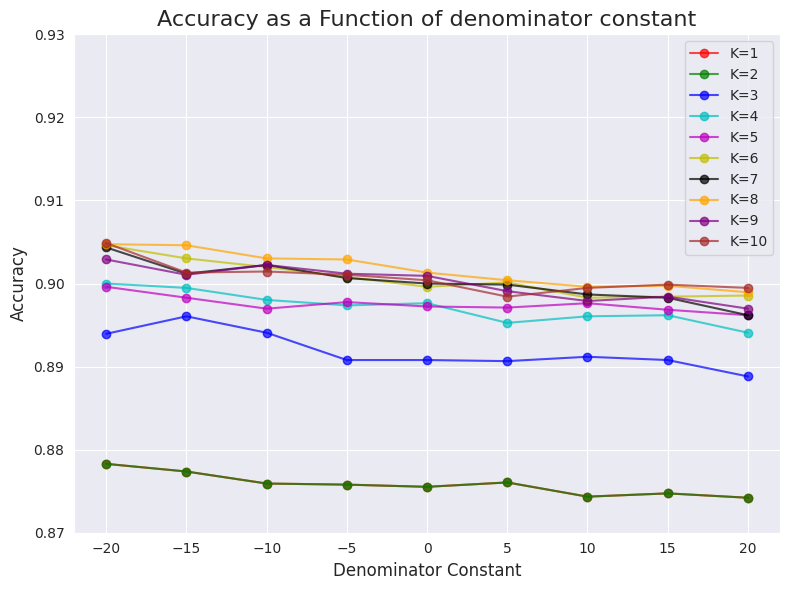
I also tested it with higher constants (in increments of 20):
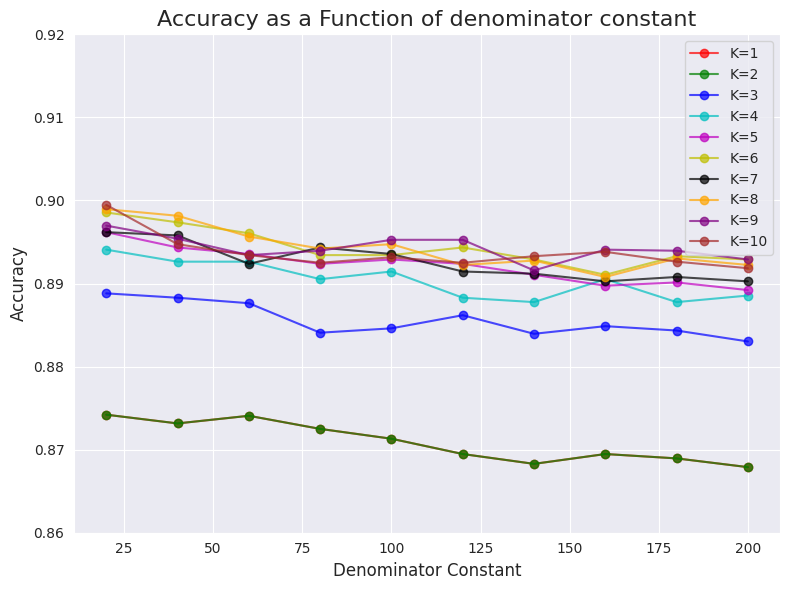
You can see that in general, the higher the constant the lower the accuracy. This makes me suspect that the authors of the paper could have actually received slightly better results 🤗.
Summary
I’m still not completely bought by this method, so I would probably still prefer to use BERT (or any other LLMs for that matter) over this method.
But still, I really liked how the authors took a step back from the usual trend of “let’s build a bigger model” and thought out a somewhat competitive algorithm for BERT.
I’m excited to see what the future holds for new approaches like this, and I hope we see more papers like this one challenging the norms.
Hope you enjoyed this post.
Until next time,
Tal